The faster local model run took 83x longer

On 2026-08-04 I sent the same local model request twice, 30 seconds apart. The first run reported 188.16 tokens per second. The second reported 153.12. The first run took 43.9 seconds of wall clock. The second took half a second.

Tokens per second picked the wrong winner by 23%. Wall clock says the second run was 83 times faster.

Both runs were llama3.1:8b on an RTX 5090 through Ollama, same prompt, 44 input tokens and 32 output tokens, num_ctx=1024. The 188.16 tok/s run spent 43,476.3 ms in its load phase and 170.06 ms generating. Tokens per second measures the generating part only, so it hid 99% of what the request actually cost.

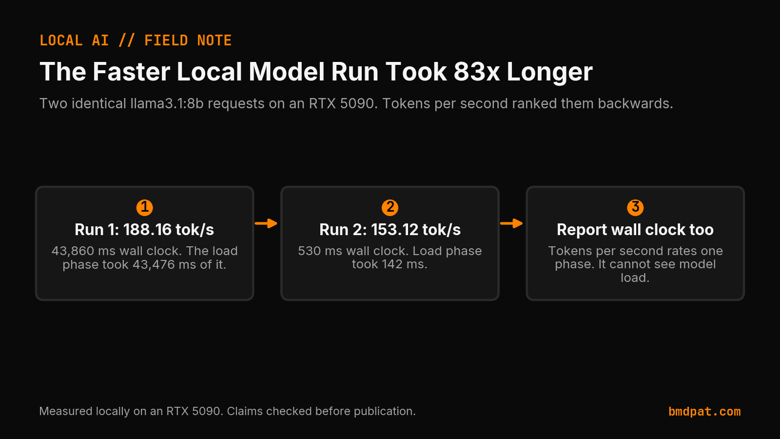
What did the two runs actually measure?

Same model, same prompt, same settings. Here is what the receipt recorded.

Do the division and both speed numbers check out. 32 tokens over 170.06 ms is 188.2 per second. 32 tokens over 208.98 ms is 153.1. Neither number is wrong. They answer a question I was not asking.

Why does tokens per second rank the runs backwards?

Tokens per second divides output tokens by generation time. Ollama reports that generation time as eval_duration, and it reports load_duration and prompt_eval_duration as separate fields. The API documents all three.

So the metric is a rate for one phase of the request. It cannot see the other two.

In the first run the load phase was 43,476.3 ms of a 43,832.66 ms total. That is 99.2% of the request. The rate for the remaining 0.8% led the table.

This is not a rounding problem. For a 32 token answer, generation is the smallest part of the job. Ranking a short agent call by generation rate ranks it by the part that barely matters.

What does the receipt say about the gap?

The receipt records the load phase and the memory delta. GPU memory went from 855 MiB to 5,994 MiB across the first request and stayed at 5,994 across the second. The weights arrived during the first call.

I am not going to write "cold start" into the artifact. The runner stamps residency_state=unrecorded on both rows, and I keep a rule that the label comes from the receipt and not from my reading of it. That rule came out of an earlier fix to the same benchmark, covered in the phase timing receipt post. The measured facts are the load duration and the memory delta. Those are enough to act on, and they do not require me to invent a field.

A second row in the same report shows this is not a one-off. A qwen3.5:9b request at 77.59 tokens per second recorded 63,791 ms of wall clock for 64 output tokens. At that rate the generation accounts for about 0.8 seconds. The other 63 seconds sit in the receipt as wall clock and appear nowhere in the headline speed.

What should a local benchmark report instead?

Report wall clock beside tokens per second, and let the selection step read wall clock.

Three rules I now apply.

First, record all three phases. Load, prompt eval, and generation. Ollama returns them, so keeping them costs nothing.

Second, match the metric to the workload. For a batch job that generates thousands of tokens against a model already in memory, generation rate is the right number. For a single-shot agent decision returning 32 tokens, it is close to noise. My workload is the second kind.

Third, keep both runs. Do not drop the slow one as a warm-up. The first run is the honest measure of what the first request of the day costs, which is the same reason I benchmark input and output sizes separately instead of reporting one blended rate.

The change to my benchmark is small. It now reports wall clock per request next to the rate, and the row that leads on rate no longer wins by default. For an agent that makes one call and waits, 43.9 seconds is the number a person feels. 188.16 tokens per second is the number that looks good in a table.

Accompanying prompt

What the prompt does: turns a local model benchmark into a wall-clock comparison so a fast generation rate cannot hide a slow request.

Copy/paste this prompt:

Copy-ready prompt

Paste the exact block into your coding agent.

No article chrome, no footnotes, no formatting drift.

Copy promptSelect text

Role: engineer benchmarking a local language model on owned hardware. Context: my rows report tokens per second, but some hide a long model load phase. Task: 1. Per row, list load, prompt eval, generation, and total wall clock. 2. Compute what percent of wall clock each phase used. 3. Rank rows by wall clock, then by tokens per second. Show where they disagree. 4. Name the metric that matches my workload and say why. 5. Name one rerun that separates load cost from generation cost. Output: a phase table, both rankings, and the rerun command. Constraints: do not invent missing fields. Keep slow rows. Do not label a run cold or warm unless the receipt records it.

10 lines/668 chars

Ready

This prompt and every other one we publish live in the free prompt library.

Copy the block above.

Get the artifact-backed local AI lab notes by email: https://bmdpat.com/5090-reports

Related reading

• My 5090 benchmark was missing the field I needed most
• Why I Benchmark Local LLM Input and Output Separately
• VRAM Fit Is Not Runtime Support